Machine Learning
[ML/데이터 전처리]Feature Selection - Wrapper
- -
728x90
Feature Select(특징 선택): 모델을 구성하기 위한 Feature을 선택하는 과정
고차원, 즉 피처가 많을 수록 데이터 포인트 간의 거리가 기하급수적으로 멀어진다. 이 Curse of Dimensionality(차원의 저주)가 일어나는데 해당 데이터로 학습을 시켰을 때 예측에서 정확도가 떨어진다.
복잡도를 감소시켜 모델의 성능을 향상시키고 처리속도를 증가시키기 위해 하는 방법 중에 하나가 Feature Select이다.
특징 선택 알고리즘은 크게 Filter, Wrapper, Embedded 3가지로 구분한다.

이 세가지 방법론을 하나만 선택해서 사용한다기보다는 같이 사용한다. (ex. Wrapper method를 사용하기 전에 Filter method를 사용)
Wrapper
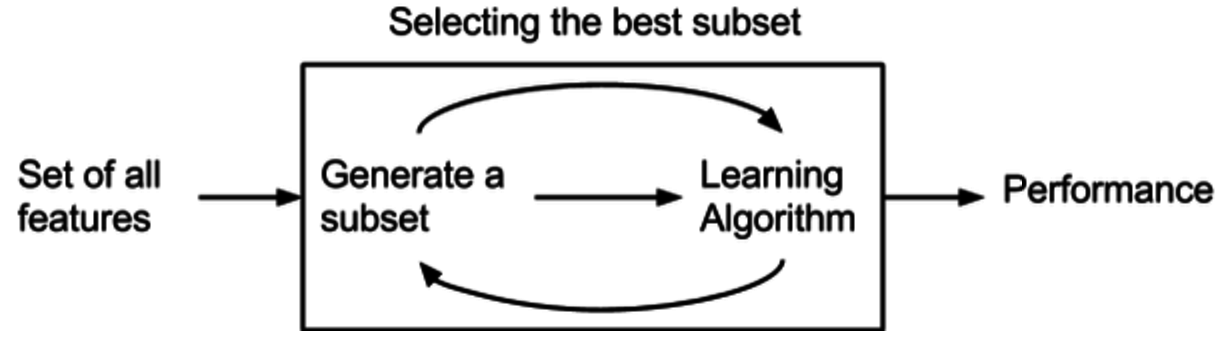
예측 정확도 측면에서 가장 좋은 성능을 보이는 Feature subset(피처 집합)을 뽑아내는 방법이다. 여러 모델을 평가해 모델의 성능을 극대화하는 최적의 조합을 찾는 방법이다. 이는 search algorithm에서 그리디 알고리즘의 개념에 따라 만들어진다.
이 경우, 기존 데이터에서 테스트를 진행할 hold-out set을 따로 두어야하고 여러번 ML을 진행하기 때문에 시간과 비용이 높게 발생한다.
Wrapper에서 사용하는 방법론
- Forward Feature Selection: 가장 유의미한 특성을 선택해나가는 방식으로 아무런 특성이 없는 상태부터 시작해서 특성을 늘려나가는 방향(Forward)으로 진행된다.
- Backward Feature Selection: 무의미한 특성을 제거해나가는 방식, 위와 반대로 모든 특성을 가진 모델에서 시작하여 특성을 하나씩 줄여나가는 방향(Backward)으로 진행된다.
- Exhaustive Feature Selection: 모든 특성 조합을 시험해보는 방식
- Step-wise Selection: 전진 선택과 후진 제거 방식을 매 단계마다 반복하여 적용하는 방식
Forward Feature Selection
전진 선택법이라고도 하며, 매 단계마다 가장 성능이 좋은 특성을 선택한 뒤에 유의미한 성능이 없을 때까지 이 과정을 실행한다.

각 단계에서 중요한 변수를 결정하는 방법
다양한 방법으로 중요한 변수가 무엇인지 결정할 수 있다. p-value가 가장 작은 값을 중요한 변수로 지정하거나, 결정계수$R^2$가 가장 많이 증가하는 변수를 지정하거나, 다른 예측 변수에 비해 loss 값이 가장 많이 감소할 때 중요한 변수로 지정할 수 있다.
언제 변수 선택을 멈출 것인지?
임계값을 정하는 방법에도 여러가지 존재한다.
- 0.05, 0.2, 0.5 등의 값을 고정적으로 정한다.
- AIC(Akaike information criterion)에 의해 결정한다
- BIC (Bayesian information criterion)에 의해 결정한다.
첫 번째 방법을 선택할 경우, 모든 변수에 대해 임계값을 정한다. 이때 임계값으로 정한 수치는 임의로 결정한 것이기 때문에 주관적일 수도 있다는 단점이 존재한다.
두 번째와 세 번째 방법에서는 AIC 또는 BIC가 임계값을 자동으로 결정하도록 하고, 각 변수마다 임계값이 달라진다.
AIC(Akaike information criterion)
AIC는 주어진 데이터 셋에 대한 통계 모델의 상대적인 품질을 평가하는 것이다. 값이 낮으면 낮을수록 좋다.
$$AIC = -2 \ln(L) +2k$$
여기서 $-2 \ln(L)$는 모델의 적합도를 의미하며, k는 모델의 추정된 파라미터 개수를 의미한다. L은 Likelihood function을 의미한다. 즉 AIC가 낮다는 것은 모델 적합도가 높다는 것을 말한다. 2k는 해당 모형에 패널티를 주기 위해 사용되었다. 실제로 어떤 모델이 적합도를 높이기 위해 여러 불필요한 파라미터를 사용할 수도 있는데 이때문에 독립변수에 따라 모형 적합도에 차이가 난다. 이를 상쇄하기 위해서 불필요한 파라미터, 즉 독립변수의 수가 증가할수록 2k를 증가시켜 패널티를 부여하여 모델의 품질을 평가하도록 했다.
AIC를 임계값의 기준으로 사용한다면 변수의 자유도(통계적 추정을 할 때 표본자료 중 모집단(x)에 대한 정보를 주는 독립적인 자료의 수)에 대한 정보를 주는 독립적인 자료의 수) 정도에 따라 임계값을 선택한다. 즉, 다시 이야기하자면 변수들간의 편향을 적게 만들어준다.
likelihood를 가장 크게 하는 동시에 변수 갯수는 가장 적은 최적의 모델을 찾게 해준다.
code
# AIC(Akaike information criterion)

import statsmodels.api as sm

def forward_feature_selection(X, y):
    selected_features = []
    remaining_features = set(X.columns)
    current_score, best_new_score = float('inf'), float('inf')

    while remaining_features and current_score == best_new_score:
        scores_with_candidates = []

        for feature in remaining_features:
            model = sm.OLS(y, sm.add_constant(X[selected_features + [feature]])).fit()
            score = model.aic
            scores_with_candidates.append((score, feature))

        scores_with_candidates.sort()
        best_new_score, best_feature = scores_with_candidates[0]

        if current_score > best_new_score:
            remaining_features.remove(best_feature)
            selected_features.append(best_feature)
            current_score = best_new_score

    return selected_features
# Forward Feature Selection 수행
selected_features = forward_feature_selection(X, y)
selected_features = pd.Series(selected_features)
print(selected_features)BIC (Bayesian information criterion)
$$BIC = -2 \ln(L) +\log(n)p$$
AIC와 유사하지만 마지막 패널티를 수정함으로써 AIC를 보완했다. 변수가 많을 수록 AIC보다 더 패널티를 가하게 되고, BIC는 Likelihood와 변수의 개수를 동시에 고려 임계값을 선택한다.
변수 개수가 작은 것이 우선 순위라면 AIC보다 BIC를 참고하는게 좋다. 표본 크기(또는 로지스틱 회귀의 경우 이벤트 수)가 독립 변수당 100을 초과하는 대규모 표본 크기로 작업하는 경우에만 권장된다. [Heinze et al.]
code
def forward_feature_selection(X, y):
    selected_features = []
    remaining_features = set(X.columns)
    current_score, best_new_score = float('inf'), float('inf')

    while remaining_features and current_score == best_new_score:
        scores_with_candidates = []

        for feature in remaining_features:
            model = sm.OLS(y, sm.add_constant(X[selected_features + [feature]])).fit()
            score = model.bic  # BIC로 변경
            scores_with_candidates.append((score, feature))

        scores_with_candidates.sort()
        best_new_score, best_feature = scores_with_candidates[0]

        if current_score > best_new_score:
            remaining_features.remove(best_feature)
            selected_features.append(best_feature)
            current_score = best_new_score

    return selected_features
# Forward Feature Selection 수행
selected_features = forward_feature_selection(X, y)
selected_features = pd.Series(selected_features)
print(selected_features)Backward Feature Selection
후진제거법이라고도 하며, 특성을 제거했을 때 가장 성능이 좋은 모델을 선택하며 유의미한 성능 저하가 나타날 때까지 이 과정을 반복한다.
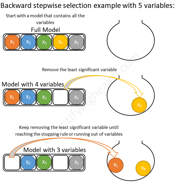
각 단계에서 삭제할 변수 선택 기준과 언제 변수 선택을 멈출 것인지는 전진선택법과 동일하다.
#aic

def backward_feature_selection(X, y):
    selected_features = list(X.columns)
    current_score = calculate_aic(X, y, selected_features)
    best_new_score = current_score

    while len(selected_features) > 1:
        scores_with_candidates = []

        for feature in selected_features:
            new_features = list(set(selected_features) - set([feature]))
            score = calculate_aic(X, y, new_features)
            scores_with_candidates.append((score, feature))

        scores_with_candidates.sort()
        best_new_score, best_feature = scores_with_candidates[0]

        if current_score > best_new_score:
            selected_features.remove(best_feature)
            current_score = best_new_score
        else:
            break

    return selected_features

def calculate_aic(X, y, features):
    model = sm.OLS(y, sm.add_constant(X[features])).fit()
    return model.aic
# bic
def backward_feature_selection(X, y):
selected_features = list(X.columns)
current_score = calculate_bic(X, y, selected_features)
best_new_score = current_score
while len(selected_features) > 1:
scores_with_candidates = []
for feature in selected_features:
new_features = list(set(selected_features) - set([feature]))
score = calculate_bic(X, y, new_features)
scores_with_candidates.append((score, feature))
scores_with_candidates.sort()
best_new_score, best_feature = scores_with_candidates[0]
if current_score > best_new_score:
selected_features.remove(best_feature)
current_score = best_new_score
else:
break
return selected_features
def calculate_bic(X, y, features):
model = sm.OLS(y, sm.add_constant(X[features])).fit()
return model.bicRecursive Feature Elimination(RFE)
대표적인 Backward elimination 방법으로 feature importance ranking에 따라 덜 중요한 Feature를 제거한다. 원하는 개수의 변수가 나올때까지 반복하는데 몇 개의 feature를 남겨야 할 지를 사용자가 직접 정의해야한다. 이 단점을 극복하기 위해서 RFECV라는 방법이 제시되었다. 가장 feature importance가 낮은 feature들을 제거해가면서 각 feature 개수마다 모델의 성능을 계산해가는데 각 feature 개수마다 K-fole validation 등의 cross validation을 활용하여 각기 다른 성능을 도출한다.
도출된 각 feature 개수별 성능을 평균내어 가장 높은 성능을 가지는 feature 개수에 해당하는 feature들을 최종 feature selection 결과로 사용한다.
RFE에서 feature importance를 계산하는 방법은 특정 피처의 값을 임의의 값으로 치환했을 때 원래 데이터보다 예측 에러가 얼마나 더 커지는가를 측정한다.

Feature Importance의 경우 해당 피처가 모델의 판단에 긍정적인 영향을 미치는지, 부정적 영향을 미치는지 알 수 없다. 또 퍼뮤테이션 전도와 에러에 기반한 추정 한계 때문에 알고리즘 실행시마다 중요도가 다를 수 있다. 또 feature 간의 의존성을 간과한다는 한계도 존재한다.
# Recursive Feature Elimination(RFE)
from sklearn.feature_selection import RFECV
from xgboost import XGBClassifier

# RFECV를 사용한 feature selection 수행
estimator = XGBClassifier()  # 사용할 모델 선택
rfecv = RFECV(estimator=estimator)
X_selected = rfecv.fit_transform(X, y)

# 선택된 특성의 논리값 리스트
selected_features = rfecv.support_

# 선택된 특성의 열 이름
selected_feature_names = X.columns[selected_features]

# 결과 출력
print("선택된 특성:")
print(selected_feature_names)
언제 전진 선택법을 쓰고, 언제 후진 제거법을 사용할까?
전진 선택법은 고려 중인 변수의 수가 샘플 크기보다 훨씬 많을 때 사용한다. feature가 없는 널 모델에서 시작하여 한 번에 하나씩 변수를 추가하기 때문에 전체 모델(모든 feature가 포함된)을 고려할 필요가 없다.
후진 제거법은 모든 변수의 효과를 동시에 고려할 수 있다는 장점이 있다. 즉 모델의 변수가 서로 상관관계가 있는 경우를 고려할 수 있다. 후보 변수의 수가 표본 크기(또는 이벤트 수)를 초과하지 않는 한, 후진 제거법을 사용한다.
Step-wise Selection
Foward Selection 과 Backward Elimination 을 결합하여 사용하는 방식이다. 모든 변수가 포함된 모델에서 출발하고 기준통계치에 가장 도움이 되지 않는 변수를 삭제하거나 모델에서 빠져있는 변수 중에서 기준 통계치를 가장 개선시키는 변수를 추가함. 이러한 변수의 추가 또는 제거를 반복한다.
참고
https://quantifyinghealth.com/stepwise-selection/
Understand Forward and Backward Stepwise Regression – QUANTIFYING HEALTH
Running a regression model with many variables including irrelevant ones will lead to a needlessly complex model. Stepwise regression is a way of selecting important variables to get a simple and easily interpretable model. Below we discuss how forward and
quantifyinghealth.com
AIC, BIC, Mallow's Cp 쉽게 이해하기
개요회귀모델에서 설명변수가 많을 경우에는 설명변수를 줄일 필요가 있습니다. 설명변수가 많으면 예측 성능이 좋지 않기 때문이죠. 많은 설명변수를 가지는 회귀분석의 경우 설명변수들사이
rk1993.tistory.com
728x90
'Machine Learning' 카테고리의 다른 글
| [ML] 분류 모델(Classification Model) (0) | 2023.07.03 |
|---|---|
| [ML/데이터 전처리]Feature Selection - Embedded (0) | 2023.06.30 |
| [ML/데이터 전처리] Feature Selection - Filter (0) | 2023.06.27 |
| [ML/DL] manifold? (0) | 2023.02.21 |
| [ML] Dimensionality Reduction #2 t-SNE, LLE (1) | 2023.02.03 |
Contents
소중한 공감 감사합니다